

Section outline
-
-
Introduction to astrochemistry
Astrochemistry, or molecular astrophysics, is the study of molecules in space. Since their first detection in the interstellar medium in the 1930's, molecules have proven to be important probes of the physical state of many astrophysical environments relevant to the lifecycle of a galaxy. For example, the formation and destruction mechanisms of molecules provide cooling mechanisms that are necessary to explain crucial processes, such as the collapse of interstellar clouds into stars. Similarly, the chemistry involved in the formation of planets is likely responsible for the emergence of life. Beyond their importance in the formation of stellar systems, chemical processes are also deeply involved in the deaths of stars. Close to the end of their life, stars similar to our sun lose most of their material through dense winds driven by dust formation, an inherently chemical process. These outflows seed the interstellar medium with fresh elements and dust grains: the building blocks of the next generation of stars and planets. Chemistry is thus irrevocably intertwined with the physical evolution of astrophysical environments.
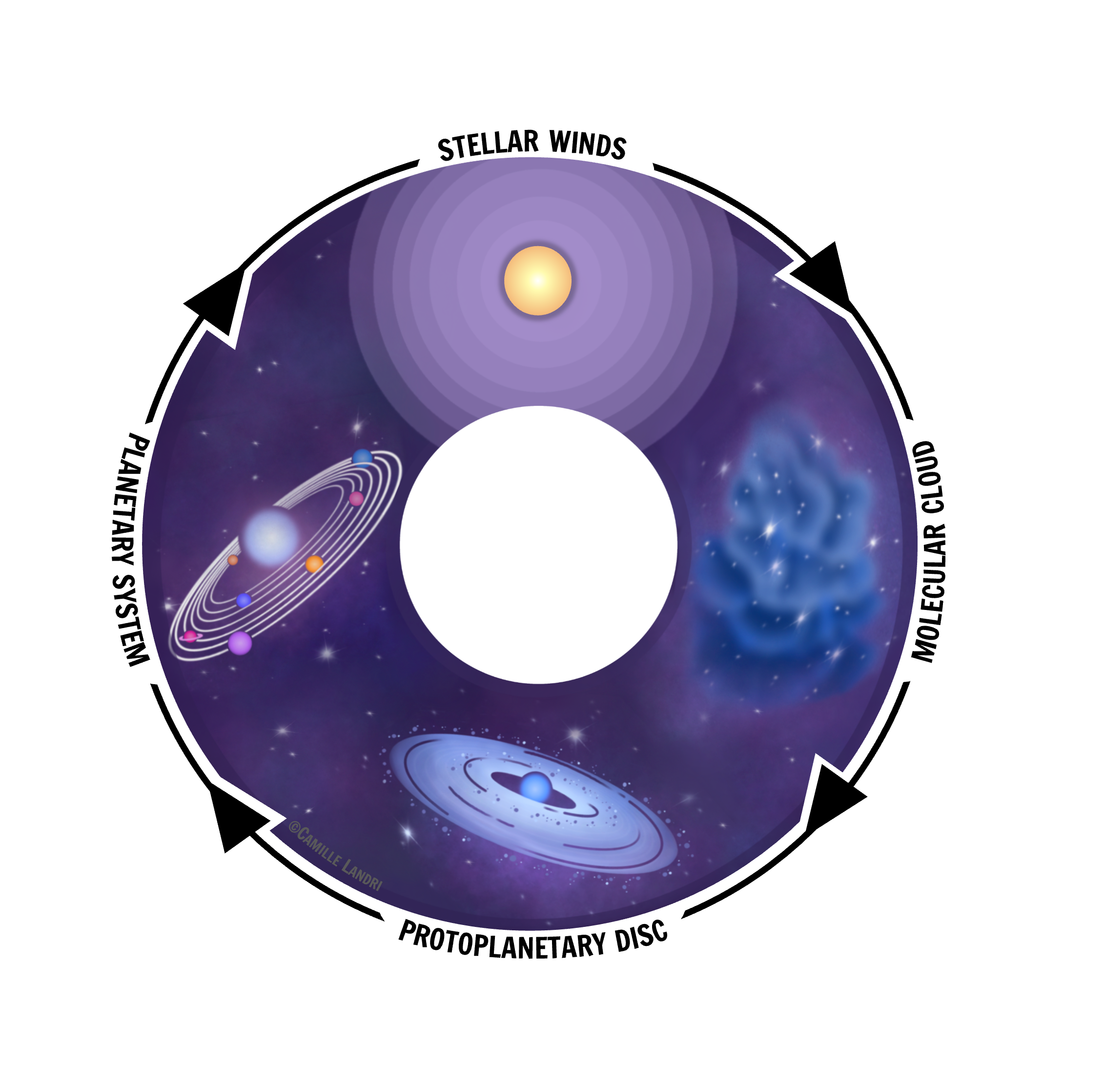
Lifecycle of stars. Stellar winds seed the interstellar medium, leading to the formation of molecular clouds.
These clouds then collapse into protostars, which accrete matter and later form of planetary systems.
-
AGB outflows
Close to their deaths, stars born with masses ranging from 0.5 to 8 times the mass of our Sun experience a phase of strong mass loss, an evolutionary stage commonly called the Assymptotic Giant Branch (AGB) phase. During this phase, a combination of pulsations and dust formation drives a stellar wind at the surface of the star, gradually stripping the star from its material, and causing a macroscopic outflow. In turn, this leads to the creation of a vast circumstellar envelope (CSE).
High resolution observations of these CSEs show that instead of being spherically symmetric, these outflows exhibit a variety of complex geometries, from spiral patterns (see image below), to disc-like structures or even random structures. These structures are thought to be due to a companion obejct orbiting the AGB star, which then interacts gravitationally with the wind and perturbs the ouflow.
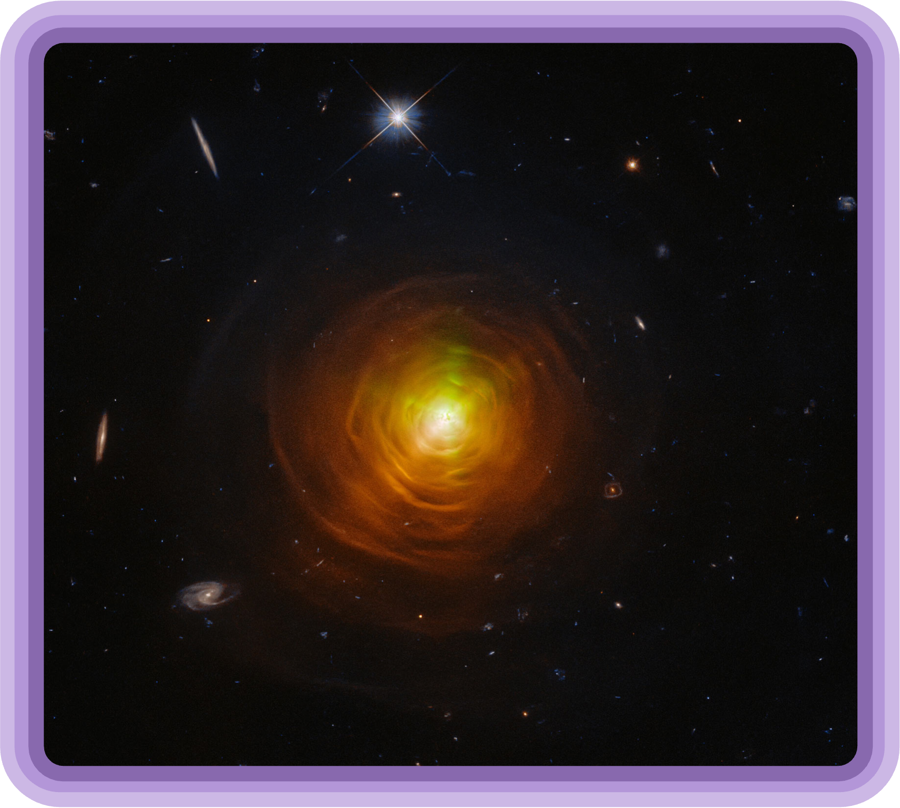
Hubble observation of the outflow around the AGB star CW Leonis (NASA/ESA).
Additionally, the CSE around AGB stars is exposed to UV radiations from the surrounding interstellar medium, which photodissociate the neutral species present in the outflow. The ions and radicals, created by the photodissociation, then allow for a rich chemical activity that forms a wide diversity of molecules. The formation of molecules depend on the physical state of the outflow, for instance the local densities, temperature and the radiation passing through the gas. Some molecules can form in denser regions of the outflow, while other may only form in the colder outer regions. Thus, observing the emission of specific molecules in AGB outflows is a crucial tool to understand better the dynamics and state of the outflow.
-
-
-
Why simulations?
Experiments in astrophysics are limited. Since we are incapable of reproducing stars or galaxies in a lab, we rely mostly on observations and simulations to test out theories. Specifically, we set up theoretical models of astrophysical environments starting from the basic laws of physics, and compare the results with observations. We can then refine the models by adding more physical processes, or expand the initial conditions to explore a larger parameter space.
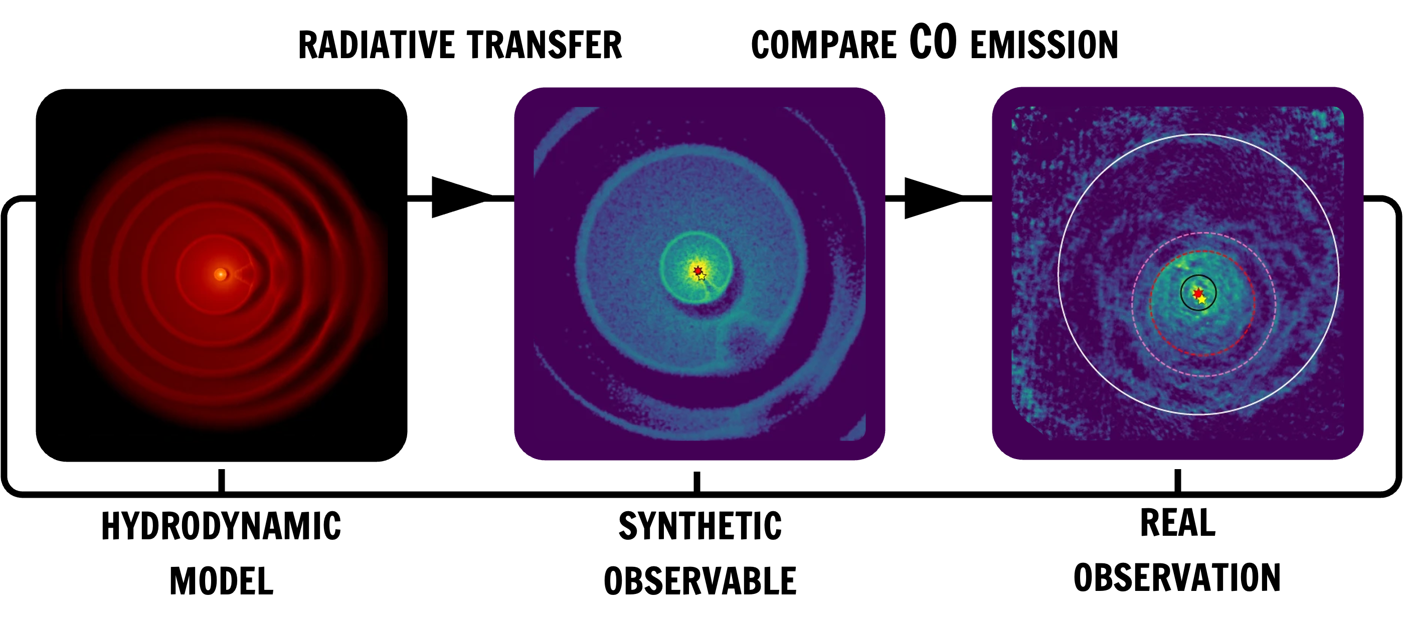
Starting from hydrodynamic model, we run radiative transfer with some assumption on chemical
abundances and obtain a spectrum, then compare this synthetic spectrum with real observations.
For environments where the interplay between chemical and physical processes is strong, such as AGB outflows, the complete astrophysical model should consist of a minimum of three building blocks. We need (i) hydrodynamics, to describe the dynamical processes of the astrophysical fluid, (ii) radiative transfer, to describe the interaction between the light and fluid, and (iii) chemistry. Ideally, these three building blocks should be incorporated into a 3D model, capable of resolving the spatial complexity of the environment.
-
Coupling chemistry and hydrodynamics
While the ideal astrophysical simulation may include hydrodynamics, radiative transfer and chemistry, issues quickly arise when considering the computational cost of each component. Hydrodynamics and radiative transfer are already computationally intensive, but incorporating chemical kinetic networks immensely increases both the memory and computational cost of the model.
When studying chemical kinetic networks, we need to solve a large number of coupled ordinary differential equations (ODEs). Since chemical reaction rates span many orders of magnitude and certain chemical processes have very short timescales, the ODEs are very stiff and should be solved over very small time steps to ensure the stability of the solutions. And naturally, the more extensive and accurate the network, the more expensive the calculation, since it should account for hundreds of chemical species which are connected by thousands of reactions. Fortunately, such a calculation takes only a fraction of a second. However, solving the set of coupled ODEs at every time step, at every position in a 3D simulation, quickly escalates to a huge amount of added calculation time to the already computationally expensive model. This renders these complete models impossibly expensive, especially if one wants to explore a reasonable part of the parameter space of the astrophysical environment we are interested in.
We thus need to be creative with finding new techniques to speed up the simulations. Different approaches have been investigated over the past decades, and the most popular ones aim to reduce the chemical network to its key species and reactions, given the environment. However, such methods require extensive parameter studies and error quantification to assess the reduced network’s performance. More importantly, by using a reduced network one runs the risk of neglecting species and/or reactions that contain vital yet unforeseen information on the physical state of the environment. Therefore, it is important to keep a full chemical network to retain a certain level of accuracy. In this specific case, we aim to incorporate a full chemical network and turn to techniques of machine learning (ML) in order to a surrogate model for astrochemistry.
-
More on astrochemical simulations
For a more detailed explanation of the complexity of astrochemical simulations, check out this video!
-
-
-
The code
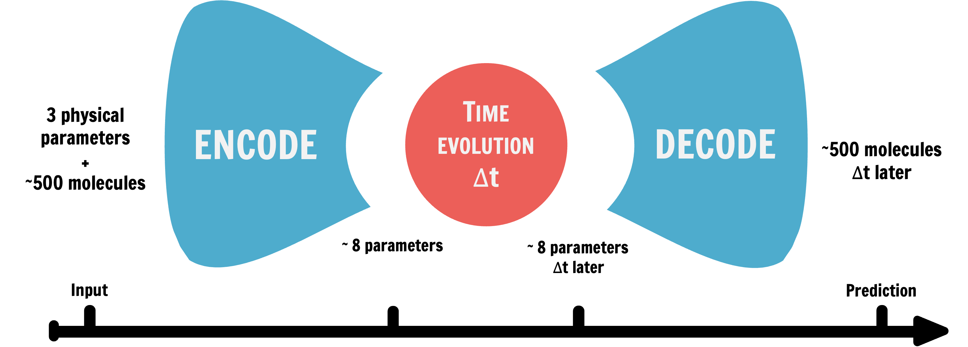
MACE stands for machine learning approach to chemistry emulation. It is an architecture trained as a surrogate model for astrochemistry, and is able to reproduce the evolution of chemical abundances in about 5% of the time its classical analogue takes. It consists of an autoencoder (encoder + decoder), which maps the input space to a latent space with reduced dimensionality and vice versa, and a trainable ODE, that solves the evolution of the “latent chemistry” over time.

The encoder and decoder are represented by a neural network and have a mirrored architecture with respect to each other. The input, i.e. the physical parameters of the environment and set of initial chemical abundances, is first mapped to its latent representation by the encoder. This latent input is then evolved over a latent time, which is connected to the physical time, by the trained latent ODE. Finally, the evolved latent state is mapped back to the dimensions of the original input by the decoder.
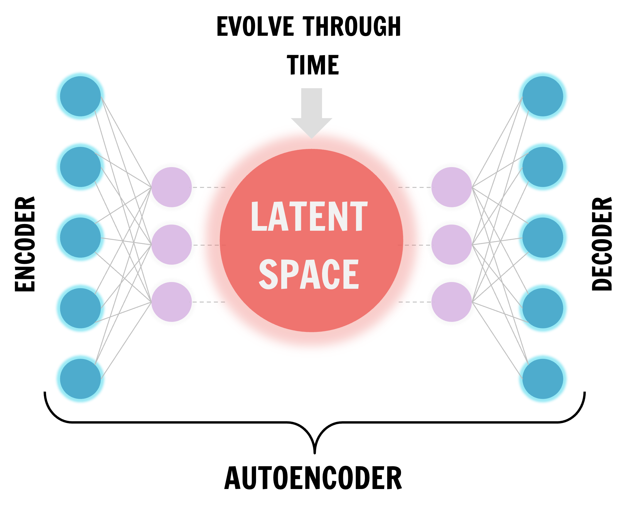
Architecture of MACE
-
Usage
MACE acts as a 0D surrogate model for chemistry. This means that the input consists of the physical parameters at a certain time/location in the simulation and the time interval of chemical evolution, together with a set of abundances (n0). MACE returns the set of abundances at the later time interval (nt).
-
More on MACE
For more information on how we built MACE, watch this video!
-
-
-
Team
Dr. Silke Maes

Sumaqua, Leuven, Belgium
Previously at the Institute of Astronomy, KU Leuven, Belgium
Dr. Frederik De Ceuster

Institute of Astronomy, KU Leuven, Belgium
Leuven Gravity Institute, KU Leuven, Belgium

Dr. Marie Van de Sande
Leiden Observatory, Leiden University, The Netherlands

Dr. Camille Landri
Institute of Astronomy, KU Leuven, Belgium

Prof. Leen Decin
Director of the Institute of Astronomy, KU Leuven, Belgium
-
Acknowledgements
Silke Maes acknowledges the support from the Research Foundation Flanders (FWO) grant G099720N.
Frederik De Ceuster is a Postdoctoral Research Fellow of the Research Foundation - Flanders (FWO), grant number 1253223N, and was previously supported for this research by a Postdoctoral Mandate (PDM) from KU Leuven, grant number PDMT2/21/066.
Marie Van de Sande acknowledges the support from the Oort Fellowship at Leiden Observatory.
Camille Landri and Leen Decine acknowledge the support from KU Leuven C1 BRAVE grant C16/23/009.
Leen Decin acknowledges the KU Leuven Methusalem grant SOUL METH/24/012, and the FWO research grants G099720N and G0B3823N.
The team is grateful for the support of DiRAC.

/prod01/prodbucket01/media/durham-university/departments-/physics/logos/dirac-logo-1740X856.png)

-